"Pictorial representation is essential for
discovery and rapid understanding" (John L. Synge).
Digital Geometry
Digital geometry −a field within discrete geometry− handles sets of digitized discrete points representing two- or three-dimensional graphs in Euclidean space. These graphs can be:
Raster.
A raster graphic, raster image or bitmap is a data structure encoded by a grid or mesh (usually two-dimensional) of pixels or colored (or grayscale) dots that can be represented on matrix devices such as displays, plotters, and printers.
A raster> image has width (a), height (h) and color depth (bits per pixel). The latter determines the number of different colors that can be stored in each pixel. With 1 bit we have 2 colors (black and white), with 2 we have 4 colors, with 4 we have 16 colors, and with 8 bits we have 256 possible colors. Colors can be additive (as in a monitor), using 3 basic colors (RGB, red-green-blue), or they can be subtractive, in which case 4 colors are used (CMYK, cyan-magenta-yellow-black).
The resolution of a raster device is the number of pixels per inch (PPI, pixels per inch).
Vector.
A vector graphic is defined by vectors. A vector is an oriented line segment defined by the coordinates of the endpoints (x1, y1) y (x2, y2). It is assumed that any shape (circle, arc, polygon, etc. can be represented by vectors. The filling of shapes can also be done by vectors.
Vector graphics have the advantage that they can be enlarged without loss of quality, unlike raster graphics. Likewise, they can be moved and transformed.
Vector graphics can be plotted on vector devices (such as plotters). To represent them on matrix devices they have to be rasterized. For this purpose a certain line width has to be assumed. The quality of the graphic depends on the resolution used.
Graphics languages
In Computer Graphics a lot of effort has been put into creating graphics standards, with different criteria. However, these standards constitute isolated languages, not connected to a general or universal language.
Graphics languages are specialized languages (such as markup languages, database management languages, etc.), based on specific graphical primitives (line, circle, etc.). There are vector, raster or both. There are static and dynamic graphics. And there are also software interface oriented languages: API (Application Program Interface). The most important ones are:
GKS (Graphical Kernel System). First ISO standard (1977) for 2D vector graphics. There is a version for 3D, GKS-3D, also ISO standard.
PHIGS (Programmer's Hierarchical Interactive Graphics System) is a standard API for rendering 3D graphics. It gave rise to OpenGL.
CGM (Computer Graphics Metafile). ISO/IEC standard. Open international standard file format for 2D vector graphics, raster graphics and text. In general, metafile formats are formats that allow vector and raster information to be included, such as CGM, PDF, SVG, RTF, EPS, PICT and CDR.
WebCGM. CGM version for the Web.
IGES (Initial Graphics Exchange Specification). ANSI standard. Format for data exchange between CAD systems.
VML (Vector Markup Language). It is a Microsoft format with XML syntax. 2D or 3D vector graphics, static or dynamic for the Web.
PGML (Precision Graphics Markup Language). Adobe Systems, Sun Microsystems.
SVG (Scalable Vector Graphics). W3C consortium standard for the Web. XML-based format for describing 2D vector graphics, static and dynamic. Can be edited with a text editor. Allows the inclusion of raster and text. SVG was born from the combination of VML and PGML.
File formats raster: JPEG, GIF, BMP, PNG, TIFF, etc.
Page description formats: PDF, PCL and PostScript. Contain text, vectors and images.
CGI Computer Graphics Interface. It is an ISO standard for interactive graphics oriented to the interface of the graphic device rather than the API. CGI provides a device-independent 2D graphics standard. CGI describes the interface between an independent device and the dependent parts of a graphics system. CGI sits between the GKS system and the graphics device.
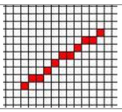
The Bresenham algorithm
The Bresenham algorithm is used to convert a vector into a set of raster points. It determines the cells of a two-dimensional grid that must be marked (drawn) to form an approximation to a straight line between two given points. It was developed by Jack Bresenham in 1962, at IBM, and published in 1965 in the IBM Systems Journal [Bresenham, 1965].
A raster vector example
Bresenham's algorithm was one of the first to be developed in the field of computer graphics because of its simplicity and effectiveness. It uses only addition and subtraction of integers and bit shifting, simple operations that all processors have. However, it is included in the processors (as hardware or firmware) of modern graphics cards.
This algorithm is commonly used to draw lines on a computer screen. The screen consists of a two-dimensional array of pixels addressable by their coordinates (x, y). It is also used in other matrix devices, such as plotters, printers, etc.
The algorithm in pseudocode
This algorithm draws a series of pixels between the points (x1, y1) y (x2, y2).
The coordinate values are integers.
Supone dx = x2−x1 > 0 and dy = y2−y1 ≤ dx. For each x between x1 and x2 the y closest to the theoretical value is chosen: that of the straight line joining both points.
The drawing matrix is assumed to be initially at zeros.
Uses an incremental error instead of division operations. That error is determined as less than or greater than 0.5 (half a pixel). Hence, Bresenham's algorithm is also referred to as the "midpoint algorithm".
Function line(x1, y1, x2, y2)
dx = x2−x1
dy = y2−y1
error = 0 // incremental error
p = dy/dx // slope of the line
y = y1
For x = x1 To x2
draw(x, y) // draw pixel in (x, y)
error = error + p
If abs(error) ≥ 0.5 Then
y = y+1
error = error−1
End If
End For
End Function
The function draw(x, y) places a numeric value in the cell (x, y), value that can be simply 1 (interpreted as "black") or an integer associated to a color (combination of some basic colors) or to a grayscale.
Function draw(x, y)
(matrix/i/j) = 1)
End Function
The following is the generalized one-line drawing function, which takes into account the possible values of dx and dy:
Function lineag(x1, y1, x2, y2)
dx = x2−x1
dy = y2−y1
Case dx = 0 Then
For y = y1 To y2
draw(x1, y) // pixel in (x, y)
End For
Case dy = 0 Then
For x = x1 To x2
draw(x, y1) // pixel in (x, y)
End For
Case dx ≥ dy Then.
line(x1, y1, x2, y2)
Case dx < dy Then.
line(x2, y2, x1, y1)
End Cases
End Function
Version in C
void MidpointLine(int x1,y1,x2,y2)
{int dx = x2−x1;
int dy = y2−y1;
int d = 2*dy−dx;
int increE = 2*dy;
int incrNE = 2*(dy−dx);
x = x1;
y = y1;
WritePixel(x, y);
while (x < x2)
{if (d<= 0)
{d+ = incrE;
x++}
else
{d+=incrNE;
x++;
y++;}
WritePixel(x, y);}
}
Variants and extensions of the Bresenham algorithm
The label "Bresenham" is used on a whole family of algorithms that extend or modify the original Bresenham algorithm. For example:
An algorithm that draws all pixels that the line touches.
An algorithm that uses grayscale [Pitteway & Watkinson, 1980].
A variant of the original algorithm is used to draw circles (Bresenham's midpoint circle algorithm).
Alan Murphy [1978] generalized the algorithm to draw thick lines.
Xiaolin Wu developed a 2-step algorithm. It implements the line drawing as an automaton (finite state machine) that observes at each step the next two pixels, where there are 12 possible configurations). It also takes advantage of the symmetry of the line, drawing simultaneously at both ends towards the center. Detailed information on this algorithm can be found in an article by Brian Wyvill in Graphics Gems [Wyvill, 1990].
MENTAL as Graphics Language
MENTAL is not only able to formalize geometric structures. It is also capable of drawing over a region of abstract space, so that, with a physical device, such space can be visualized.
MENTAL can be used as a graphical language by using a region within abstract space. The fact that the graph is independent of the representation matrix device justifies that MENTAL can be called an "abstract graphical language".
The use of Bresenham's algorithm makes it possible to implement the continuous (the vectorial) through the discrete (the matrix).
It does not need any graph language or any graph primitive, since the graphs are generated with the universal semantic primitives.
The primitive "line", which draws (at an abstract level) on a two-dimensional matrix, is sufficient. Curves (circles, arcs, ellipses, etc.) can be approximated by line segments.
The generation language of the graphic object matches the internal language of the object itself.
Integrates raster and vector.
It is device independent. It is portable, it is universal.
It is a user extensible language.
MENTAL resources allow image compression.
The use of a unified language such as MENTAL to create graphics provides great advantages, advantages derived from the possibilities of the language, with no other limit than that of the imagination. Flexibility, clarity, simplicity and creativity are maximum and go beyond graphic standards. For example:
Integrate data and graphics.
Use several graphic spaces and switch between them as required. These graphic spaces can be layers.
Interconnect graphic environments automatically, so that if certain conditions are met in one space, it changes in the others.
Define virtual graphics (composed of sub-objects of objects), generic graphics (parameterized or not), interlaced graphics, etc.
Create graphs or subgraphs depending on whether a condition is met or not.
Make reference by name to a whole chart or a part.
Create n−dimensional plots and obtain automatic projections.
Use rules to set or change attributes automatically.
Restrict drawing in certain areas.
Make selective replicas.
Assign attributes to graphical elements, graphics, spaces, etc. and then select them and perform actions.
Make animated graphics using rulers.
Grouping graphic objects.
Animated graphics.
Temporary hiding of graphic objects.
Switching of graphic objects.
Multilayer graphics.
Charts as parts of a database record.
Perform parallel processes.
Describe graphics and run them when needed.
Filter by gray levels.
Shared objects. A change in the object would affect all graphics containing it.
Assignment of variable attributes.
Assignment of variable color values.
Object hierarchies.
Integral reuse of graphics and data.
Joint parameterization of data and graphics.
Interactivity is easier.
Permanent functional relationships between graphic objects.
etc.
With MENTAL you can create specialized languages for architecture, GIS (geographic information systems), mechanical design, etc.
Some examples
Suppose we want a certain group of points to be visible or invisible, depending on the value of a variable. To those points we assign the value ⟨k⟩ (a generic expression):
( D\2 = ⟨k⟩ )


( D\6\9 = ⟨k⟩ ) ...
By making k=0, all those points would be invisible. And by making k>0, all would be visible. In general, k could be an integer indicating a color.
Location of a graphic object in a variable graphic space (array):
( ⟨E⟩= v )


( ⟨E⟩\6\9 = v ) ...
By making (E = D), the object is located in D space.
Location of the points of an object referred to a given point in 2D space (i0, j0):
( ⟨D0 = v⟩ )


( ⟨D\(i0+1)\(j0+2) = v⟩ )
Making (i0=7 j0=9) the object moves according to this reference position.
Addenda
Computational Geometry
Computational Geometry is a branch of computer science devoted to the study of algorithms that can be stated in terms of geometry. The main impetus in the development of computational geometry as a discipline was the progress in computer-generated graphics (Computer Graphics) and in applications such as CAD/CAM (computer-aided design and manufacturing), GIS (geographic information systems), CAE (computer-aided engineering) and integrated circuit design.
The two main branches of computational geometry are:
Combinatorial computational geometry, also called algorithmic geometry, which treats geometric objects as discrete entities [Preparata & Shamos, 1988].
Numerical computational geometry, also called machine geometry, computer-aided geometric design (CAGD) or geometric modeling, which deals mainly with the representation of real-world objects in forms treatable by CAD/CAM systems. This branch can be considered a further development of descriptive geometry and is often considered a branch of computer graphics or CAD [Forrest, 1971].
Bibliography
Angell, Ian O. Gráficos con computador. Paraninfo, 1986.
Bernstein, Saúl; McGarry, Leo. Arte por ordenador. Cómo pintar y dibujar con su Ordenador Personal. Ediciones CEAC, 1989.
Bresenham, Jack E. Algorithm for computer control of a digital plotter. IBM Systems Journal, vol. 4, no. 1, pp. 25–30, Enero 1965.
Chauveau, Karla Steinbrugge; Chin, Janet S.; Reed, Theodore Niles. The Computer Graphics Interface. Butterworth-Heinemann, 1991.
Flanagan, Colin. The Bresenham Line-Drawing Algorithm. Internet.
Forrest, A.R. Computational geometry. Proc. Royal Society London, 321, series 4, 187-195, 1971.
Klette, Reinhardt; Rosenfeld, Azriel. Digital Geometry. Geometric Methods for Digital Picture Analysis. Morgan Kaufmann, 2004.
Lewell, John. Aplicaciones gráficas del ordenador. Panorama de las técnicas y aplicaciones actuales. Hermann Blume, 1986.
Mark Friedhoff, Richard; Benzon, William. Visualization. The second computer revolution. W.H. Freeman and Company, 1989.
Miller, Frederic P.; Vandome, Agnes F.; McBrewster, John (editores). Digital geometry: Discrete space, Euclidean space, Image analysis, Computer graphics, Bresenham's line algorithm, Pick'stheorem, Mathematical morphology. Alphascript Publishing, 2010.
Murphy, Alan. Line Thickening by Modification to Bresenham's Algorithm. IBM Technical Disclosure Bulletin, vol. 20, no. 12, pp. 5358-5366, Mayo 1978. Disponible en Internet con el título “Murphy's Modified Bresenham Line Drawing Algorithm. An Algorithm for drawing thickened lines”.
Preparata, Franco P.; Shamos, Michael Ian. Computational geometry. An introduction. Springer, 1988.
Sproull, Robert F. Using program transformations to derive line-drawing algorithms. Technical Report, Dept. of Computer Science, Carnegie-Mellon University, 1981 (17 páginas).
Varios autores. Computer Graphics Algorithms: Bresenham's Line Algorithm, Flood Fill, Painter's Algorithm, Ray Tracing, Scanline Rendering, Alpha Compositing. Books LLC, 2010.
Wyvill, Brian. Symmetric Double Step Line Algorithm. In A. Glassner (editor) Graphic Gems, pp. 101-104, Academic Press, 1990.